One of the things I liked about old paper spreadsheets was the fact that ever other row was highlighted, making it much easier to read. Until it added conditional formatting, this was something that had to be done manually in Excel, i.e. select every other row and change the background color. While this worked, whenver a row was inserted or deleted, one had to repeat the process.
With the advent of conditional formatting it is relatively easy to highlight alternate rows. Here are the steps:
Select the area in which you wish to highlight alternate rows.
Go to the Format menu and select Conditional Formatting.
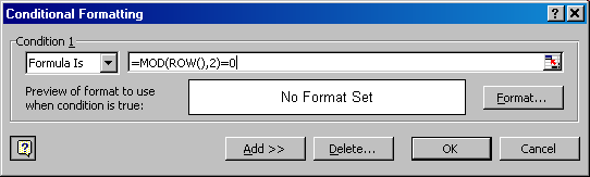
In Condition 1, in the leftmost box, select "Formula Is"
In the right box, type in "=MOD(ROW(),2)=0" if you wish to highlight every even row, or type "=MOD(ROW(),2)=1" if you wish to highlight every odd row. See the image below:
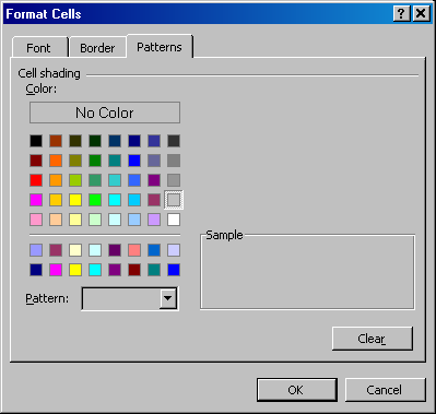
Then click on the Format button. When the Format dialog box pops up, click on the Patterns tab.
Select the background color and pattern you wish to apply to your alternate rows. The image below shows selecting light gray for the background.
Click OK on the Format dialog box. Then click OK on the Conditional Formatting dialog box.
The area you selected should have every other row showing the background you selected
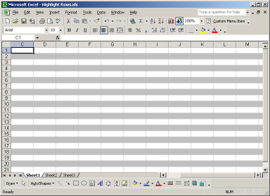
The sample below was creating by simply selecting the entire worksheet and following the above steps:
The nice thing about this method is that if you add or delete a row, the shading remains consistent.